
Forensics Challenge Day Two - Sleuth Kit Deep Dive
Welcome back for day two! Today will be all about "Disk and File System Analysis" - read the series' first part if you want to know what's going on and on which book we are working :D
Understanding Media and File System Analysis in Digital Forensics
Digital forensic analysis can feel like diving into a vast, invisible world inside your storage devices. To navigate it, we need a solid understanding of what we’re looking at, how it’s structured, and how to extract useful evidence. Let's walk through it step by step.
What is Media Analysis in Digital Forensics?
Imagine you're a digital archaeologist. Instead of pottery or fossils, you're digging through hard drives, memory cards, and SSDs. You’re looking for files: some visible, some deleted, some hidden within others.
Media analysis is the process of:
- Identifying what files and data exist or used to exist.
- Extracting relevant content and metadata.
- Analyzing what all that means in context.
These steps may seem linear, but in practice, they often overlap. For example:
File carving (a recovery technique) involves identifying file signatures in raw data and pulling out file content; so it’s both identification and extraction.
Analogy:
Think of it like cleaning out an old attic.
- Identification is opening boxes and labeling what’s inside.
- Extraction is pulling out items of interest.
- Analysis is understanding the story these items tell: who lived here, when, what happened?
File System Abstraction Model: The Layers of the Digital World
To make sense of what we find on a disk, we use something called the File System Abstraction Model. Think of it as a map: or better yet, the OSI Model of storage, where we go from the physical up to what users actually interact with.
Let’s break down each layer with examples and analogies:
1. Disk: The Physical Foundation
This is the actual hardware: a hard drive, SSD, USB stick, or SD card. Just like your house sits on the ground, everything digital sits on a disk.
Example: A 1TB SATA hard drive.
Forensics here is very advanced: think clean rooms and microscopes. Not the everyday examiner’s job.
Fun Fact: Traditional disks store data in sectors of 512 bytes; newer ones often use 4096-byte sectors.
2. Volume – The Disk's Neighborhoods
A volume is a slice (or multiple slices) of a disk. You might know these as partitions. For example:
- Your
C:andD:drives (on Windows) are different volumes. - A USB stick with one partition is one volume.
Note: "Partition" = on one disk; "Volume" = may span multiple disks.
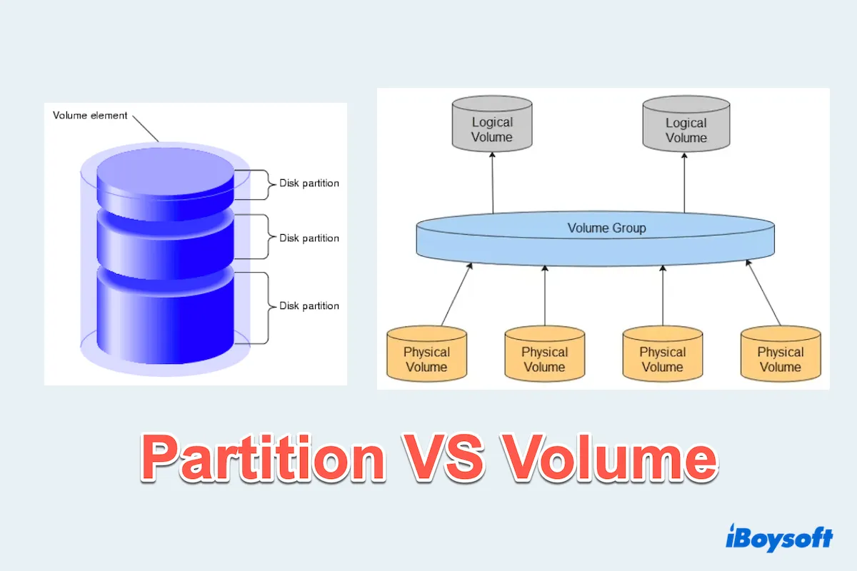
Analogy:
Think of the disk as a cake. A partition is one slice. A volume might be one slice, or multiple slices stuck together to form a layer cake.
3. File System – The Filing Cabinet Inside the Volume
The file system organizes how data is stored and retrieved. It’s like the indexing system of a giant digital library.
Examples: NTFS, FAT32, Ext4.
It keeps track of where files are, their sizes, timestamps, and more.
Without a file system, a volume is just raw data.
4. Data Unit – The Smallest Building Block
Data units are the basic chunks of data storage inside a file system. Often called blocks (especially in Unix), these are where actual content lives.
- If a file is a book, then data units are its pages.
- If a data unit is assigned to a JPEG file, it stores part of that image.
Sizes vary: Data units are often 4KB on modern systems.
| Unit | Typical Size | Description |
|---|---|---|
| Block | 4 KB | Most common default on modern systems (e.g., NTFS, ext4). |
| Cluster | 4–64 KB | Often synonymous with block, especially in Windows. Larger sizes can be used for large volumes. |
| Sector | 512 B or 4 KB (Advanced Format) | Physical unit on the disk. File systems operate on top of this. |
| Page (in memory) | 4 KB | Related to how OS handles memory-mapped files. |
5. Metadata – Data About the Data
Metadata tracks information about files, not their actual content.
Example: Created on June 12, owned by Alice, size = 512KB. Unix-based systems use inodes (Index Nodes) to store metadata.
Analogy: If the file is a package, metadata is the shipping label.
6. File Name – What We See
This is the layer where humans interact with files.
holiday\_photo.jpgbudget.xlsx
But behind each name is a pointer to the metadata and content.
File names can be misleading. Just because something’s called report.docx doesn’t mean it’s actually a Word document.Important Caveats
This model is best suited to Unix-like systems. Windows and other systems might implement things differently, but the core concepts generally map over. Not all examiners go down to the disk level. Most work at the volume, file system, or metadata layers.
Want to Go Deeper?
For those ready to get their hands dirty with hex views, journal entries, and inode parsing, the bible of this field is:
“File System Forensic Analysis” by Brian Carrier
TL;DR
| Layer | What It Represents | Analogy |
|---|---|---|
| Disk | Physical storage hardware | The ground/foundation |
| Volume | Logical chunk(s) of storage | Slices of cake |
| File System | The organization method | Filing cabinet/library index |
| Data Unit | The smallest storable unit | Book pages / Lego bricks |
| Metadata | Info about the data | Shipping labels |
| File Name | Human-readable file/directory names | Folder labels |
Now, let's talk about what we can do on the different levels - here come the tooools.
Introducing The Sleuth Kit: Your Forensic Toolbox
When you're diving into forensic file system analysis, you're going to need a reliable set of tools. And The Sleuth Kit (TSK) is just that: a Swiss Army knife for digital archaeologists.
What Is The Sleuth Kit?
Originally developed by Brian Carrier, TSK is the modern successor to an older Unix toolset called The Coroner’s Toolkit (TCT). While TCT was great for its time, it had a few big problems:
- It only really worked on Unix-like systems.
- It wasn’t portable across platforms.
- It didn’t support newer or non-Unix file systems.
TSK fixed all that. It’s:
- Cross-platform
- Open source
- Actively maintained
- Modular and extensible
Installing The Sleuth Kit (And Why You Might Want to Compile It Yourself)
TSK supports raw disk images out of the box. But if you want to process images in formats like EWF (Expert Witness Format) or AFF (Advanced Forensic Format), you’ll need support from external libraries: LibEWF and AFFLib.
You can usually install TSK via your system’s package manager. But here’s the kicker:
Compiling from source gives you:
- The latest version (repos can lag behind)
- Full control (no middlemen)
- Immediate feedback during configuration (so you know what features are enabled)
Success Checklist
In the first part, we talked a lot about this, if you want to catch up about ./configure
When you run the configuration script, check for these lines to confirm that support for image formats is active. Let's go through installation together
wget https://github.com/sleuthkit/sleuthkit/releases/download/sleuthkit-4.14.0/sleuthkit-4.14.0.tar.gz
tar xzf sleuthkit-4.14.0.tar.gz
cd sleuthkit-4.14.0

ls
---
aclocal.m4       ChangeLog.txt  docs         Makefile.am  packages          tests       win32
API-CHANGES.txt  config         INSTALL.txt  Makefile.in  README.md         tools
bindings         configure      licenses     man          README_win32.txt  tsk
case-uco         configure.ac   m4           NEWS.txt     samples           unit_tests
---
Then we can continue like descripbed in the last post:
./configure
In the output, I find (yours may differ):
checking for afflib/afflib.h... no
checking for libewf.h... yes
checking for libewf_get_version in -lewf... yes
and fix that "no" with:
sudo apt install afflib-tools libafflib-dev
so for now we're left with:
configure:
Building:
   afflib support:                        yes
   libewf support:                        yes
   zlib support:                          yes

   libbfio support:                       yes
   libvhdi support:                       no
   libvmdk support:                       no
   libvslvm support:                      no
Features:
   Java/JNI support:                      no
   Multithreading:                        yes
seems good enough. Finish it with:
make
sudo make install
And you're done. TSK is now installed.
Heads Up: Root Access Required
If you're targeting a live, attached disk (not just a forensic image), you’ll need root privileges.
Use either:
sudo <command>su -to switch to root entirely (NOT RECOMMENDED!! BE CAREFUL!)
Otherwise, access to protected disk structures will be blocked.
Understanding TSK's Tool Naming Structure
With 21+ command-line tools, TSK might seem overwhelming at first. But there’s a method to the madness.
TSK uses prefixes and suffixes in tool names that tell you:
- What layer of the file system the tool operates on
- What the function of the tool is
Sleuthkit Prefixes – What Layer Are You Operating On?
| Prefix | Layer | Example Tool | Description |
|---|---|---|---|
mm- | Volume Layer | mmstat | Media management tools |
fs- | File System Layer | fsstat | File system metadata and layout |
blk- | Data Unit (Block) Layer | blkls | Shows raw block content |
i- | Metadata (Inode) Layer | istat | Metadata inspection |
f- | File Name Layer | fls | Lists files/directories by name |
j- | Journal Layer | jls | Lists contents of file system journal |
img- | Image Tools | img_stat | Works on disk image files |
Suffixes – What Does the Tool Do?
| Suffix | Function | Example Tool | Description |
|---|---|---|---|
-stat | Show stats/info | istat | Like Unix stat, shows metadata |
-ls | List contents | fls | Like Unix ls, lists files or blocks |
-cat | Dump content | icat | Like Unix cat, outputs raw file data |
Not Everything Fits the Pattern
Some miscellaneous tools in TSK don’t follow this naming scheme, but don’t worry, they’re documented separately. We’ll stick to the core tools for now, progressing layer by layer.
TL;DR Summary
| Topic | Key Idea |
|---|---|
| The Sleuth Kit (TSK) | A powerful, open-source forensic toolkit from Brian Carrier |
| Compiling vs Installing | Compiling gives latest version and control over dependencies |
| Tool Structure | Prefix = Layer, Suffix = Function |
| Next Up | Volume Layer Tools (mm- prefixed commands) |
Volume Layer Tools: Understanding What Lies Beneath
In digital forensics, analyzing a disk image means understanding how storage is structured before you can dig into what’s stored.
The first structural layer we can look at is the volume layer, and The Sleuth Kit (TSK) gives us tools with the prefix mm- to help explore this.
What’s a Volume System?
When you plug in a hard drive, it may contain multiple partitions; these are logical chunks of space that the OS can use. The way these partitions are described is handled by the volume system.
A volume is like a district within a city. It defines the borders where the file system begins and ends. When a disk has multiple partitions (likeC:andD:on Windows), these are each volumes, possibly with different file systems (e.g., NTFS, ext4).
When you're analyzing disk images, understanding volume structure is crucial. If you can’t locate the right volume, your deeper analysis (files, metadata, etc.) is pointing at the wrong district.
Two common volume systems are:
| Name | Description | Analogy |
|---|---|---|
| MBR (Master Boot Record) | Older format (pre-UEFI). First 512 bytes of the disk contain the partition table and bootloader. | A classic filing cabinet with labeled drawers. |
| GPT (GUID Partition Table) | Modern standard (used with UEFI). Supports more partitions, bigger disks. | A modern database-backed cabinet with more structure. |
We'll dig deeper into MBR/GPT later on. For now, just know they're partitioning methods that describe where volumes are on a disk.
TSK Tools for Volume Layer Exploration
Let’s walk through the main tools available for volume analysis using Sleuth Kit.
mmstat: Identify the Volume System
mmstat diskimage.dd
This command tries to detect if the image has a known volume system, like MBR or GPT.
But what if you get no output?
That means the image has no partitioning scheme. It’s just a raw volumel; in other words, it starts directly with a file system like ext4, ntfs, or fat32.
💡 Example: I ranmmstat task1.imgand got nothing, butfile task1.imgreturned something.
mmstat task1.img # no output

file task1.img
task1.img: Linux rev 1.0 ext4 filesystem data, UUID=2f8a53f8-aadf-4607-8b36-188eecc92864 (needs journal recovery) (extents) (64bit) (large files) (huge files)
That means: your image is a file system image, not a disk image.
So instead of using mmstat or mmls, you’ll use file system tools like fsstat, fls, and icat directly - we'll come to them in this post, in a later section.
.img vs .dd: What's the Difference?
Technically: nothing, structurally.
| Extension | What It Usually Means | Contains |
|---|---|---|
.dd |
"Disk Dump" (raw sector-by-sector clone of a physical disk) | Full disk image, including MBR/GPT, volumes, unallocated space |
.img |
Often used for partition or file system images | May skip the partition table, starts directly with file system |
In practice, the file extension is just a convention: use the file command to understand the real structure:file image.dd
file image.imgmmls: View Volume Layout (If Present)
mmls diskimage.dd
This tool parses the partition table, showing all volumes present and their offsets (starting sector positions). Here's an example output:
Slot    Start       End         Length      Description
00:     Meta        0000000000  0000000000  0000000001  Primary Table (#0)
01:     -----       0000000000  0000000062  0000000063  Unallocated
02:     00:00       0000000063  0000096389  0000096327  NTFS (0x07)
03:     00:01       0000096390  0000192779  0000096390  NTFS (0x07)
This tells us:
- There are two volumes, both formatted as NTFS.
- There's unallocated space before and after them; maybe worth exploring later.
mmls is great because it:
- Works with both MBR and GPT
- Shows gaps and slack space
- Gives sector offsets needed for other tools like
fls,icat,fsstat, etc.
mmcat: Extract a Volume (If Needed)
If you want to carve out a single partition for focused analysis, mmcat is your tool.
mmcat diskimage.dd 02 > ntfs_volume.dd
This streams the raw contents of volume #02 (from mmls) to a new file, which you can then mount, hash, or process with tools like Autopsy or X-Ways.
Only useful if your image has a volume system — for single-volume images like the previous task1.img, just work on it directly!TL;DR – Volume Layer in Practice
| Tool | Use Case | When to Use |
|---|---|---|
mmstat | Identify volume system (MBR, GPT, etc.) | On full disk images, not raw file systems |
mmls | View partition layout, find volume offsets | When you need to know where volumes begin |
mmcat | Extract one volume to a separate file | For focused analysis on one partition |
Always verify the type of image you’re working with before choosing a tool:
file image.img
- If it says e.g. "ext4 filesystem", it's a raw file system image → skip
mm-tools, go straight tofs-. - If it says "DOS/MBR" or "GPT", it's a disk image → use
mmstat,mmls, etc.
What’s Next?
Since your image is a raw ext4 file system, we’ll jump straight into the file system layer tools next.
File System Layer Tools (fs-)
We'll learn how to:
- Inspect file system structure with
fsstat - See file/directory listings with
fsls - And much more.
Let’s keep digging. The next level is where the real story of the data begins to unfold.
File System Layer Tools – Where Structure Meets Story
Once you’ve found a volume (or you’re given a raw file system image, like the previous task1.img), the next step in digital forensics is to understand the file system: the digital logic that organizes how data is stored, retrieved, and linked together.
Wait, What Is a File System, Really?
A file system is a method an operating system uses to:
- Organize files and folders
- Track where data physically lives
- Store metadata (timestamps, permissions, etc.)
- Manage access to that data
Think of it as a librarian and index system rolled into one:
- The data blocks are the actual books.
- The metadata (like inodes) are the catalog cards.
- The file system keeps the entire library in order.
Common File Systems You’ll Encounter
| File System | Common In | Key Traits |
|---|---|---|
| Ext3 | Legacy Linux distros | Journaling, stable but outdated |
| Ext4 | Modern Linux systems | Better performance, supports large files |
| NTFS | Windows systems | Rich metadata, journaling, compression |
| FAT32 | USB sticks, SD cards | Simple, portable, lacks journaling |
| exFAT | Cross-platform USB | Successor to FAT32, better file size support |
Tip: Each file system leaves behind different types of artifacts. Ext3/4 has inodes and journaling. NTFS has MFT entries and alternate data streams. Your toolset (like TSK) must understand these structures to extract the full story.
fsstat: X-Ray Vision for File Systems
fsstat gives you metadata-rich details about the file system. Think of it as a forensic x-ray: it won’t show the files themselves yet, but it tells you how everything is laid out.
Let’s walk through a real example from an Ext4 file system:
An Example: fsstat on an Ext4 File System
Let’s look at a real-world example you might encounter in a forensic investigation. Here's what you get when running:
fsstat task1.img
This image is an Ext4 file system, one of the most common in Linux environments in 2025. We'll break it down into chunks and highlight only the most forensically relevant pieces. Not every line is useful, but some are goldmines for timeline building, anomaly detection, or hidden evidence.
General File System Info
File System Type: Ext4
Volume ID: 6428c9ec8e18368b746dfaaf8538a2f
Last Written at: 2025-05-30 09:49:26 (EDT)
Unmounted properly
Last mounted on: /home/kali/mnt_task1
Source OS: Linux
Why it matters:
- Last Written / Last Mounted: Great for timeline building. Can show last system activity, or post-incident tampering.
- Unmounted properly: If
no, that may mean a crash, forced power-off, or intrusion. - Mount Path (
/home/kali/...): Hints at where the volume was last mounted useful if you suspect device reuse or cross-mounting.
Compatibility Features
Compat Features: Journal, Ext Attributes, Resize Inode, Dir Index
InCompat Features: Filetype, Needs Recovery, Extents, 64bit, Flexible Block Groups
Read Only Compat Features: Sparse Super, Large File, Huge File, Extra Inode Size
Why it matters:
- These flags tell you what structures and behaviors this FS supports.
- Ext4-specific flags like
extentsand64bitshow it can handle very large files and modern storage. Needs Recoveryflag means the journal might contain changes that weren’t committed; interesting in cases of unexpected shutdowns or malicious tampering.
Metadata Summary (Inodes)
Inode Range: 1 - 12825
Root Directory: 2
Free Inodes: 12812
Inode Size: 256
What this tells us:
- Inodes are the metadata containers for files: timestamps, permissions, etc.
- Only 13 inodes are used, which means the file system is nearly empty.
- Root inode is 2: always the case in Ext filesystems.
Forensics tip: If few inodes are in use but a lot of blocks are allocated, the rest could be data without links — maybe leftovers from deleted files!
Content Summary (Blocks)
Block Size: 1024
Free Blocks: 42805 out of 51200
Why it matters:
- Small block size (1KB) means the image was probably created on a small system (e.g., VM, embedded device, live USB).
- High number of free blocks = lots of unallocated space, ideal for data carving.
Block Group Info (Short Summary)
This section shows the internal subdivision of the file system into "block groups", which improve performance and help spread out file metadata.
Here’s how to read it without going crazy:
| Group | Free Inodes | Free Blocks | Notable |
|---|---|---|---|
| 0 | 98% | 56% | Contains actual directories |
| 1–6 | 100% | 87–100% | Mostly empty |
Takeaways:
- Only Group 0 has data — other groups are unused.
- Total Directories = 2 in Group 0 — likely just
/and maybe one more (like/lost+found).
🎯 Target block group 0 for further analysis: That’s where actual file data is likely stored.
📌 Why Show All This?
You don’t need to memorize every field. The forensic skill is in spotting useful signals:
- Used vs free inodes/blocks → tells you how full or wiped the file system is.
- Last mounted/written → helps build an activity timeline.
- Block size → critical when carving deleted data.
- Which group(s) contain real data → saves time when investigating large images.
TL;DR – Interpreting fsstat Output
| Element | What It Means | Why It Matters |
|---|---|---|
| File System Type | ext4, NTFS, etc. | Tells you how to interpret metadata |
| Last Written/Mounted | Timestamps | Key for incident timelines |
| Free Inodes/Blocks | How full the FS is | Indicates deletion or "freshly formatted" |
| Root Directory | Inode 2 | The entry point to the file tree |
| Block Size | Allocation unit size (e.g., 1024) | Critical for carving and low-level access |
| Block Group Layout | Physical distribution of data | Helps narrow your investigation scope |
Listing and Extracting Files with fls and icat
Now that we’ve mapped the structure of the file system with fsstat, it’s time to get our hands dirty and see what’s actually inside.
We’ll use:
flsto list all files and directories (even deleted ones!)icatto extract files by inode number
Let’s go step by step with a real example from the Ext4 image task1.img.
Step 1: Use fls to List File System Contents
fls -r -m / task1.img
The -r flag makes it recursive, and -m / sets the output paths to start from root.
Here’s part of the output:
0|/file.doc       |13|r/rrw-r--r--|0|0|0|1748612966|...|
0|/file.docx      |14|r/rrw-r--r--|0|0|0|1748612966|...|
0|/hello.py       |19|r/rrw-r--r--|0|0|15|1748612966|...|
0|/image1.png     |20|r/rrw-r--r--|0|0|224566|...|
0|/test.pdf       |25|r/rrw-r--r--|0|0|13264|...|
0|/test.txt       |26|r/rrw-r--r--|0|0|5|...|
How to read this:
| Field | Meaning |
|---|---|
13, 14, ... | Inode number — unique ID for the file |
r/rrw-r--r-- | File type and permissions |
/test.txt | File path (relative to /) |
5 | File size in bytes (for /test.txt) |
| Last columns | Timestamps (ctime, mtime, atime, crtime) |
Pro tip: When investigating, look for:
- Suspicious or unexpected files
- Zero-byte files (
size = 0): may be placeholders - Timestamps that stand out or match attack timelines
Step 2: Use icat to Extract a File by Inode
Let’s say you want to extract /test.txt, which corresponds to inode 26.
icat task1.img 26 > test.txt
Then read it with:
cat test.txt
🎯 In this case, it outputs:
hello
Boom, recovered🎉.
💡 You just extracted a file directly from its inode, skipping the file system directory structure entirely. This is key for working with deleted or orphaned files.
Special Case: $OrphanFiles
You may have noticed this line:
0|/$OrphanFiles|12825|V/V---------|0|0|0|0|0|0|0
This is the inode table overflow area. If you see actual files listed under $OrphanFiles, it often means:
- The file was deleted, but data may still be recoverable.
- The file wasn’t linked to any directory, e.g. created by malware or dumped by a script.
Explore it further with a focused fls call or by walking the inode range manually.TL;DR – fls and icat Cheatsheet
| Tool | What it does | Example Usage |
|---|---|---|
fls | Lists files + metadata from image | fls -r -m / task1.img |
icat | Extracts a file by inode number | icat task1.img 26 > test.txt |
Next Up: Data Unit Layer (blk- Tools)
With file listings and extractions under your belt, it’s time to go one layer deeper, to the raw data level.
Next, we’ll explore tools like:
blkls– list raw unallocated blocksblkcat– view raw block content- How to carve files from unallocated space
Get ready to find evidence where the file system has "forgotten", but the data still lingers...
Data Unit Layer Tools: The Rawest View of the Disk
We’re now diving to the lowest level of structured analysis: individual blocks (or data units) within the file system.
These tools are powerful when:
- You're trying to recover data from unallocated space
- You suspect anti-forensics techniques have unlinked files without wiping blocks
- You want to inspect file remnants, piece-by-piece
Reminder: In Linux-style file systems (like ext4), "blocks" are the smallest chunks of disk space used to store data. These are what files are broken down into when written.
Wait – Can I Use This on task1.img?
Not really. Here's why:
task1.imgis a raw file system image from a small volume with minimal data and almost no unallocated space.- The content is clean, nearly empty, and hasn't gone through meaningful usage that would leave behind deleted fragments or overwritten blocks.
So these blk- tools make the most sense when working with large, used images, like:- Internal HDD images from a suspect’s machine
- USB drives that have been in long-term use
- Android dumps with years of chat/media deletions
Overview of Data Unit Layer Tools (Prefix: blk-)
| Tool | Purpose | When to Use |
|---|---|---|
blkstat | Shows info about a single block | Check if a block is allocated or not |
blkls | Lists/extracts all unallocated blocks | Before carving deleted data |
blkcat | Reads and outputs a specific block | Inspect raw content manually |
blkcalc | Maps offset in unallocated dump → image | Trace back what file a fragment came from |
blkstat: Is This Block Allocated?
blkstat disk.img 521
Example output:
Fragment: 521
Allocated
Group: 0
Use this when:
- You want to confirm whether a specific block is in use or free
- You’re trying to validate block group structures in ext filesystems
blkls: Dump All Unallocated Space
blkls disk.img > disk.unalloc
This grabs all unallocated blocks from the file system and saves them to one file; a prime target for data carving (e.g., with foremost, scalpel, binwalk).
Example:
foremost -i disk.unalloc -o output_dir
Use when:
- You suspect deleted files that aren’t in the inode table anymore
- You want to scan for file signatures (PDF, JPG, DOCX) in free space
blkcat: View Raw Block Contents
blkcat disk.img 521 | xxd | head
This outputs the raw hex and ASCII representation of block 521.
Use when:
- You're analyzing a suspicious file or directory block
- You want to verify data encoding or file signatures
Example output snippet:
0000020: 6c6f 7374 2b66 6f75 6e64 0000 0c00 0000  lost+found.....
0000030: 1400 0c01 2e77 682e 2e77 682e 6175 6673  ......wh..wh.aufs
You can literally read the block and find strings like "lost+found" or ".wh.aufs" embedded inside it.
blkcalc: Reverse Map to Original Image
Let’s say you find something interesting in your blkls dump, and you want to know:
Where did this block come from in the original image?
That’s where blkcalc shines.
blkcalc disk.img -b 521
Use when:
- You’re analyzing an extracted block (e.g. from
foremostorstrings) - You want to trace a fragment back to its physical location
TL;DR – When to Use blk- Tools
| Scenario | Tool(s) You Need | Goal |
|---|---|---|
| Want to confirm if a block is used | blkstat | Allocated vs. unallocated |
| Want to carve deleted file remnants | blkls, foremost | Grab & scan unallocated space |
| Want to see what’s inside a block | blkcat, xxd | Raw hex/ASCII view of data |
| Want to trace a block back to image | blkcalc | Understand where fragment came from |
Use Case Snapshot: Carving from Unallocated Space
Imagine this scenario:
You're investigating an image from a USB drive. You suspect someone deleted incriminating PDFs. Here's what you'd do:
blkls usb.img > usb.unalloc
foremost -i usb.unalloc -t pdf -o pdfs/
Within minutes, you may have recovered plans.pdf, completely bypassing the file system structure.Metadata Layer Tools – Investigating the Who, When, Where
Metadata is where a huge part of forensic magic happens.
At this layer, we’re looking at inodes (in Linux/Unix file systems like Ext3/Ext4); small but powerful structures that hold:
- Who owns a file
- When it was created, modified, deleted
- How big it is
- Where its data blocks are stored
In essence: files lie, metadata doesn’t.
💡 Think of inodes like index cards in a library. The book (file content) can be torn out, renamed, or moved. But the card (inode) still records when it was added, who checked it out, how many pages it had, and where it was stored.
istat: Inspect a Single Inode in Detail
This command gives a detailed breakdown of one file’s metadata.
istat task1.img 26
inode: 26
Allocated
Group: 0
Generation Id: 799561121
uid / gid: 0 / 0
mode: rrw-r--r--
Flags: Extents,
size: 5
num of links: 1

Inode Times:
Accessed:       2025-05-30 09:49:26.039381649 (EDT)
File Modified:  2025-05-30 09:49:26.039381649 (EDT)
Inode Modified: 2025-05-30 09:49:26.039381649 (EDT)
File Created:   2025-05-30 09:49:26.039381649 (EDT)

Direct Blocks:
8720
What this tells you:
| Field | Value / Explanation |
|---|---|
uid / gid | 0 / 0 : The file was owned by the root user and root group |
mode | rrw-r--r-- : Regular file, owner can read/write; group/others can read only |
Flags | Extents : Used in Ext4 to manage large files more efficiently |
size | 5 : The file is 5 bytes in size (likely something like hello) |
num of links | 1 : Only one directory entry points to this inode |
Accessed | 2025-05-30 09:49:26.039381649 : When the file was last read |
File Modified | 2025-05-30 09:49:26.039381649 : When the content was last changed |
Inode Modified | 2025-05-30 09:49:26.039381649 : When the metadata was last changed (e.g. chmod) |
File Created | 2025-05-30 09:49:26.039381649 : Creation time (Ext4 only!) |
Deleted | Not shown : Indicates the file is still allocated / not deleted |
Direct Blocks | 8720 : This is where the 5 bytes of content are stored on disk |
In Ext4, the presence of the “File Created” timestamp is a helpful enhancement over older filesystems like Ext3, which didn’t store file creation times (crtime). For forensic timelines, this is a big win.
Tip: If Deleted time is 1969-12-31, it usually means the file is still allocated and not deleted.
Use Case:
Want to prove that a file was tampered with after creation? istat gives you the timestamps to build that case.
ils: Listing All Inodes: From Structure to Story
While istat tells you everything about one inode, ils lets you look at every inode. Think of it as dumping the entire inode table of the file system. This is your best friend for broad analysis, timeline construction, and scanning for deleted or unlinked files.
ils Example
ils -aZ task1.img
This shows all:
-a: Allocated inodes (still active files)-Z: Inodes that have been used at least once (ctime ≠ 0)
Here's a shortened version of what I got:
st_ino | st_alloc | st_uid | st_gid | st_mtime   | st_atime   | st_ctime   | st_crtime  | st_mode | st_nlink | st_size
2      | a        | 0      | 0      | 1748612966 | 1748612966 | 1748612966 | 1748612966 | 755     | 3        | 1024
11     | a        | 0      | 0      | 1748612966 | 1748612966 | 1748612966 | 1748612966 | 700     | 2        | 12288
20     | a        | 0      | 0      | 1748612966 | 1748612966 | 1748612966 | 1748612966 | 644     | 1        | 224566
26     | a        | 0      | 0      | 1748612966 | 1748612966 | 1748612966 | 1748612966 | 644     | 1        | 5
12825  | a        | 0      | 0      | 0          | 0          | 0          | 0          | 0       | 1        | 0
How to Read This:
| Column | Meaning |
|---|---|
st_ino | Inode number — the unique ID of a file in the file system |
st_alloc | a means the inode is currently allocated (file still exists) |
st_uid/gid | Owner (User ID / Group ID), often 0 = root |
st_mtime | File content modified time (epoch) |
st_atime | File accessed time |
st_ctime | Inode changed time (permissions, ownership, etc.) |
st_crtime | File creation time (only present in Ext4 and newer FS) |
st_mode | File type and permission bits (like ls -l) |
st_nlink | How many file names link to this inode |
st_size | File size in bytes |
Practical Takeaways From This Output:
- Inode 2 → likely the root directory (
st_mode755,st_nlink3, size 1024) - Inodes 13–26 → various user files (like
file.doc,test.mp3, etc.) - Inode 12825 → appears to be
$OrphanFiles, empty but allocated (filesystem-dependent) - All timestamps are identical, indicating files were created and written in a bulk operation or test environment
st_size = 0→ many files were created but have no content (e.g. test cases or placeholders)
💡 In live investigations, divergent timestamps, unlinked but allocated inodes, or inode-only data remnants are often goldmines for forensic insights.
What Can I Do with This?
Here’s where ils becomes a central tool:
For Timeline Construction:
Pipe the output into a bodyfile format for use with mactime:
ils -a -m task1.img > bodyfile.txt
mactime -b bodyfile.txt > timeline.csv
This builds a human-readable CSV timeline of file activity — perfect for building forensic narratives.
For Finding Lost or Deleted Files:
Use flags like -A for unallocated inodes (deleted files), or -p for orphaned inodes (unlinked, no directory entry):
ils -A task1.img          # Show unallocated (deleted) files
ils -p task1.img          # Show orphaned (potentially hidden) files
For Cross-Matching:
Once you spot an interesting inode (e.g., inode 20):
- Use
istatto inspect it deeply - Use
icatto extract its content - Use
flsto find its file name (if any) - Use
ifindto trace block ↔ inode relationships
icat: Extract Content by Inode
You’ve seen this before, but here’s why it belongs in this layer:
icat task1.img 20 > recovered.doc
This pulls data directly from the inode, bypassing filenames or directory structure.
Why it’s powerful:
- You can recover deleted files even if they’re unlinked
- You can extract orphaned files or fragments
- You can automate mass extraction based on inode lists
ifind: Find Which File References a Block or Inode
ifind -d 28680 task1.img
This tells you which inode owns a given block (like 28680 in this case).
Alternatively:
ifind -n /hello.py task1.img
This gives you the inode number for a named file.
When to use:
- You find a juicy block with
blkcat, and want to trace it back to a file - You’re building a file-block mapping for timeline or carving validation
Putting It All Together: Metadata Workflow
Let’s say you find something suspicious:
- You run
fls, spot a filesecret.docxwith inode 20 - Use
istat task1.img 20to get timestamps - Use
icatto extract the file - Cross-reference with
ilsto see other files modified around same time - Use
ifind -don blocks to see if deleted files reused old storage
TL;DR – Metadata Tools Summary
| Tool | What It Does | Common Use Case |
|---|---|---|
istat | Inspect one inode (ownership, time, blocks) | Build timeline, confirm deletion, link to user |
ils | List all inodes | Timeline generation, deleted file hunting |
icat | Extract file content by inode | Recover deleted or unlinked files |
ifind | Map block → inode or name → inode | Trace file/block relationships |
File Name Layer Tools: fls, ffind & Building the Human View
At this layer, we move from “machine-level” views like blocks and inodes to what we actually see as users: file names and paths.
These tools let you trace names back to inodes, explore deleted entries, and generate timeline data. Think of this layer like the library index of a filesystem: titles, not contents.
I'll include fls to make everything clear.fls: List File Names (Allocated & Deleted)
Allocated Entries (Everything “Live”)
fls -r -p task1.img
Which gave this output:
d/d 11: lost+found
r/r 13: file.doc
r/r 14: file.docx
r/r 15: file.ppt
r/r 16: file.pptx
r/r 17: file.xls
r/r 18: file.xlsx
r/r 19: hello.py
r/r 20: image1.png
r/r 21: image2.jpg
r/r 22: index.html
r/r 23: test.mp3
r/r 24: test.mpeg
r/r 25: test.pdf
r/r 26: test.txt
V/V 12825: $OrphanFiles
How to Read This:
| Entry | Type | Inode | Name |
|---|---|---|---|
r/r | Regular | 20 | image1.png |
d/d | Directory | 11 | lost+found |
V/V | Virtual | 12825 | \$OrphanFiles |
The $OrphanFiles entry is a virtual folder used by Sleuth Kit to group metadata entries with no filename links. More on this below..
Deleted Files?
fls -d -r -p task1.img
... got no output. That means:
- No deleted file entries exist with name records
- However, deleted inodes may still exist — they’ve simply lost their name pointers
We’d catch those with ils -A, istat, or ffind — we’ll come back to that.
Timeline-Ready Output
fls -r -m / task1.img > bodyfile.txt
Sample bodyfile line:
0|/file.doc|13|r/rrw-r--r--|0|0|0|1748612966|1748612966|1748612966|1748612966
Fields:
| Field | Meaning | |
|---|---|---|
13 | Inode number | |
r/rrw-- | File type + permissions | |
| `0 | 0` | UID / GID |
0 | File size | |
| Last 4 | mtime, atime, ctime, crtime (Unix epoch) |
This is used as input for:
mactime -b bodyfile.txt > timeline.csv
ffind: Find File Name from Inode
Use ffind to look up filenames from inode numbers — the reverse of fls.
ffind task1.img 20
Result:
/image1.png
This tells you:
- Inode 20 maps to the file
/image1.png - It’s still linked in the filesystem (i.e. not deleted or orphaned)
If ffind returns nothing, that inode is likely:
- Deleted (no name entry exists)
- Orphaned (file lost directory linkage)
- Never linked (a temp or partially written file)
Summary Table
| Tool | Purpose | What You Did |
|---|---|---|
fls | List files (with inodes) - shown previously | Showed live entries in task1.img |
ffind | Find file from inode | Found image1.png from inode 20 |
fls -d | Show deleted files | None found (but might still exist in inodes) |
fls -r -m | Generate bodyfile for timeline | Created bodyfile.txt |
Sleuth Kit Power Tools: Real-World Analysis Beyond the Basics
So far, we’ve covered the classic Sleuth Kit layers: volume, file system, metadata, file names, and data units. But there’s a set of tools that don't fit neatly into those categories, yet they become essential in practical forensic workflows.
This is what I call the Power Tools toolbox.
We’ll walk through them with real examples from my analysis of task1.img, so you see how they fit into your workflow and why they’re powerful.
mactime: Build a Forensic Timeline
For timelines, I first generated a bodyfile from the file name layer using fls:
fls -r -m / task1.img > bodyfile.txt
This created a flat text file with pipe-delimited metadata — exactly what mactime expects. Here’s a snippet:
0|/file.doc|13|r/rrw-r--r--|0|0|0|1748612966|1748612966|1748612966|1748612966
0|/test.txt|26|r/rrw-r--r--|0|0|5|1748612966|1748612966|1748612966|1748612966
Then, I generated a timeline CSV using:
mactime -b bodyfile.txt -d > timeline.csv
Now you’ve got a sortable, filterable timeline of file access, modification, and creation: critical for spotting activity windows or attacker behavior.
You can open this in Excel or a log analysis tool like Timesketch.
Why it matters: It’s your forensic “storyboard.” You see when files appeared, changed, or were accessed. A spike of file modifications? That could mean exfiltration prep or malware activity.
sigfind: Spot Hidden Files by Signature
Some files don’t come with names — or even metadata. They just hide in unallocated space.
That’s where sigfind comes in.
Files like PDFs start with specific hex signatures. I used sigfind to look for %PDF (25 50 44 46) at 4096-byte boundaries:
sigfind -b 4096 25504446 task1.img
It returned:
Block: 722
Block: 1488
Block: 1541
...
Each of those blocks could be the start of a lost PDF. You can follow up with blkcat, icat, or carve with scalpel.
Why it matters: Signature carving lets you hunt down files that escaped typical file system tracking, think deleted reports, password dumps, or payloads.
hfind: Fast Hash Lookup
If you're using NSRL or a malware hash set, you’ll need to check whether files match known good or bad hashes.
Instead of grepping a massive text file, hfind queries indexed hash sets:
hfind -i nsrl.mdb md5hash
Why it matters: Hashing lets you quickly rule out known-good files or flag known malware: automating triage and reducing noise.
sorter: Extract and Sort Files by Type
sorter will extract files and sort them based on their type (not just extension). You can combine it with hash lookups too.
For example:
sorter -f ext4 -d extracted_files task1.img
Now you've got a folder of categorized files (images, documents, scripts, etc.) ready to inspect or hash.
srch_strings: Lightweight String Search
If you don’t want to install binutils just to run strings, srch_strings is built into Sleuth Kit:
srch_strings -t d task1.img | grep "password"
It outputs string matches with timestamps — useful when searching for indicators in memory dumps or carved data.
When These Tools Shine
These aren’t your first-pass tools, but they’re the ones that close cases:
- Timeline analysis shows when suspicious events happened
- Signature searching uncovers hidden or deleted files
- Sorter and hfind streamline triage of extracted data
- srch_strings gives fast insight into dumped text data
Use them when:
- You're deep in an investigation and need context
- You suspect data hiding or tampering
- You want to automate triage and focus on relevant artifacts
Image Layer & Journal Tools — Wrapping It All Up
As we round off this deep dive into Sleuth Kit tools, there are two final components that don't quite fit into the file system layers, but still deserve your attention when working real cases:
- The Image File Layer, where your
.img,.dd, or.affcontainer lives - The File System Journal, where change history can leave behind powerful remnants
Let’s unpack both, briefly but clearly, and end with why they matter.
Image File Layer: Metadata About the Metadata
Once you've captured a disk or partition, you’re usually working with an image file. That container format itself can sometimes carry valuable metadata about the acquisition.
To check what’s embedded in the image, I ran:
img_stat task1.img
But since task1.img is a raw image, the output was minimal — no embedded hashes, creator info, or case metadata.
If I were using something like AFF, I would’ve seen output like:
Image Type: AFF
Size in bytes: 629145600
MD5: 717f6be298748ee7d6ce3e4b9ed63459
Creator: afconvert
Acquisition Date: 2009-01-28 20:39:30
Why it matters: AFF and EWF (E01) formats often contain chain of custody data, hashes, and investigator notes. Even if not critical to the case findings, they support integrity and documentation.
To convert a forensic container into a raw stream, there's also:
img_cat image.aff > image.raw
Journal Layer: The Hidden History
If the file system you're analyzing supports journaling (like Ext3/Ext4, NTFS, HFS+), then it stores recent changes in a dedicated area before committing them fully.
This journal might hold:
- Deleted files
- Overwritten content
- System crash remnants
To look into it, I used:
jls task1.img
This lists the contents of the journal (if one exists).
To extract a specific journal entry:
jcat task1.img [journal_block]
Note: Not all images will have active or accessible journal content, but when they do, it can be a goldmine of residual forensic artifacts.
Final Thoughts: When These Tools Matter
While img_stat, jls, and jcat might not be daily drivers, they show their value in:
- Verifying integrity of container files
- Reviewing acquisition metadata for reports
- Finding transient or overwritten data via the journal
And that’s the full sweep of Sleuth Kit’s layered architecture: from media structures down to the journaled whisper of a deleted file.
Next up: Going into Partitioning and Disk Layouts, Hashing, Carving.. and much more
See you next time!
No spam, no sharing to third party. Only you and me.


Member discussion